
Python Package Installation Analysis: May 2024
Project Overview
I’ve recently started a new project to track package installations in Python. My goal is to create a monthly report or newsletter with the trending packages and general trends and behaviors in package installs. With this new project, we have the opportunity to gain valuable insights into the Python package landscape.
Data Source
For this project, I’m utilizing the powerful Google BigQuery public dataset. Read more about the dataset here. I’m currently running a query on Google Cloud, downloading the data as a CSV, and then analyzing it in Python in this GitHub repository. The use of these robust tools ensures the accuracy and efficiency of our data analysis.
May 24: EDA Findings
Find the analysis notebook here
Since May was the first month I queried the data and had no insights on the MoM trends, I initiated an Exploratory Data Analysis (EDA) on the dataset. This involved analyzing the distribution of package installs, which led to some interesting findings about the most used packages.
The Dataset
Below is a sample of the dataset used to analyze the data. There are 2 columns:
- Project: the name of the package
- Installs: How many times this package was downloaded in May
| Project | Installs |
|---|---|
| boto3 | 1,388,601,787 |
| botocore | 645,035,046 |
| urllib3 | 533,921,148 |
| requests | 485,817,094 |
| wheel | 474,966,050 |
Summarizing the Data
I’ve split the projects into buckets based on the number of installs.
| Bin | projects_count | projects_installs | projects_installs_pct |
|---|---|---|---|
| (0, 1] | 11,043 | 11,043 | 0.00% |
| (1, 10] | 9,507 | 38,229 | 0.00% |
| (10, 100] | 241,675 | 11,623,831 | 0.03% |
| (100, 1000] | 212,489 | 67,274,154 | 0.17% |
| (1000, 10000] | 49,432 | 144,526,470 | 0.36% |
| (10000, 100000] | 12,661 | 401,882,649 | 1.01% |
| (100000, 1000000] | 4,492 | 1,399,147,950 | 3.52% |
| (1000000, 1388601787] | 2,058 | 37,677,185,601 | 94.90% |
This table presents data on projects and their corresponding installation counts categorized into different bins based on the number of installations. Here’s a description of the table:
- Bin: This column represents the range of installations per project. Each bin range is represented as an interval, such as (0, 1], (1, 10], (10, 100], and so on.
- projects_count: This column shows the number of projects falling within each bin range. For instance, there are 11,043 projects in the (0, 1] range, 9,507 projects in the (1, 10] range, and so forth.
- projects_installs: This column indicates the number of installations corresponding to the projects within each bin range. For example, there are 11,043 installations in the (0, 1] range, 38,229 installations in the (1, 10] range, and so on.
- projects_installs_pct: This column displays the percentage of total installations represented by the projects within each bin range. For instance, projects within the (0, 1] range represent 0.00% of the total installations, projects within the (1, 10] range represent 0.00%, and so forth.
Concentration of Installations
While most projects fall into the lower installation ranges, a significant portion of the total installations is concentrated in projects with higher installation counts. For instance, projects with over 1,000,000 installations represent 94.90% of the total installations despite being only 2,058 projects.
Long Tail Distribution
The distribution follows a long tail pattern, where a few projects with extremely high installation counts contribute to a large portion of the total installations. Most projects have relatively low installation counts, while a small number have very high installation counts.
Pareto Analysis
Pareto Analysis, often referred to as the 80/20 rule or the principle of factor sparsity, is a technique used to prioritize efforts. It states that, for many outcomes, roughly 80% of the consequences come from 20% of the causes. We can apply this analysis to the provided data to identify which installation ranges contribute to most installations.
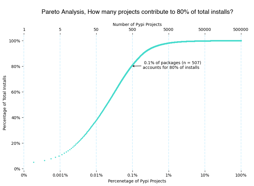
This chart illustrates a Pareto Analysis, which is a graphical representation showing how many PyPI projects contribute to 80% of the total installs. The x-axis represents the percentage of PyPI projects, plotted on a logarithmic scale ranging from 0.001% to 100%. The y-axis shows the cumulative percentage of total installs, spanning from 0% to 100%.
Key insights from the chart include:
The analysis reveals a significant imbalance in the distribution of installs across projects. A small fraction of packages (0.1% or 507 packages) accounts for a disproportionately large share (80%) of total installs. This highlights the dominance of a few highly popular packages in the PyPI ecosystem, while the majority of projects contribute to a smaller proportion of total installs.
Stay tuned for more insights and detailed reports on Python package trends and behaviors. Your feedback and suggestions are always welcome as we continue to explore the fascinating world of Python packages.
